Is Replicability in Economics better than in Psychology?

Colin Camerer and colleagues recently published a Science article on the replicability of behavioural economics. ‘It appears that there is some difference in replication success’ between psychology and economics, they write, given their reproducibility rate of 61% and psychology’s of 36%. I took a closer look at the data to find out whether there really are any substantial differences between fields.

Commenting on the replication success rates in psychology and economics, Colin Camerer is quoted as saying: “It is like a grade of B+ for psychology versus A– for economics.” Unsurprisingly, his team’s Science paper also includes speculation as to what contributes to economics’ “relatively good replication success”. However, such speculation is premature as it is not established whether economics actually displays better replicability than the only other research field which has tried to estimate its replicability (that would be psychology). Let’s check the numbers in Figure 1.

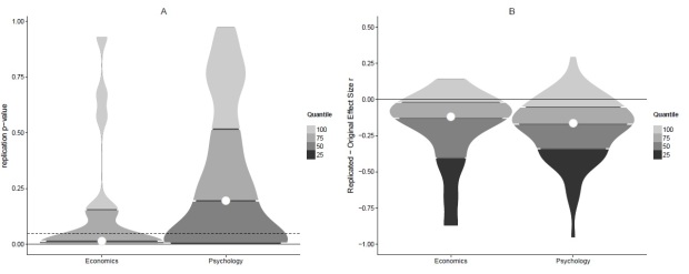
Figure 1. Replicability in economics and psychology. Panel A displays replication p-values of originally significant effects. Note that the bottom 25% quartile is at p = .001 and p = .0047 respectively and, thus, not visible here. Panel B displays the effect size reduction from original to replication study.Violin plots display density, i.e. thicker parts represent more data points.

Looking at the left panel of Figure 1, you will notice that the p-values of the replication studies in economics tend to be lower than in psychology, indicating that economics is more replicable. In order to formally test this, I define a replication success as p < .05 (the typical threshold for proclaiming that an effect was found) and count successes in both data sets. In economics, there are 11 successes and 7 failures. In psychology, there are 34 successes and 58 failures. When comparing these proportions formally with a Bayesian contingency table test, the resulting Bayes Factor of BF₁₀ = 1.77 indicates that the replicability difference between economics and psychology is so small as to be worth no more than a bare mention. Otherwise said, the replicability projects in economics and psychology were too small to say that one field produces more replicable effects than the other.

However, a different measure of replicability which doesn’t depend on an arbitrary cut-off at p = .05 might give a clearer picture. Figure 1’s right panel displays the difference between the effect sizes reported in the original publications and those observed by the replication teams. You will notice that most effect size differences are negative, i.e. when replicating an experiment you will probably observe a (much) smaller effect compared to what you read in the original paper. For a junior researcher like me this is an endless source of self-doubt and frustration.

Are effect sizes more similar between original and replication studies in economics compared to psychology? Figure 1B doesn’t really suggest that there is a huge difference. The Bayes factor of a Bayesian t-test comparing the right and left distributions of Figure 1B supports this impression. The null hypothesis of no difference is favored BF₀₁ = 3.82 times more than the alternative hypothesis of a difference (or BF₀₁ = 3.22 if you are an expert and insist on using Cohen’s q). In Table 1, I give some more information for the expert reader.

The take-home message is that there is not enough information to claim that economics displays better replicability than psychology. Unfortunately, psychologists shouldn’t just adopt the speculative factors contributing to the replication success in economics. Instead, we should look elsewhere for inspiration: the simulations of different research practices showing time and again what leads to high replicability (big sample sizes, pre-registration, …) and what not (publication bias, questionable research practices…). For the moment, psychologists should not look towards economists to find role models of replicability.

Table 1. Comparison of Replicability in Economics and Psychology.
	Economics	Psychology	Bayes Factora	Posterior median [95% Credible Interval]1
Independent Replications p < .05	11 out of 18	34 out of 92	BF10 = 1.77	0.95 [-0.03; 1.99]
Effect size reduction (simple subtraction)	M = 0.20 (SD = 0.20)	M = 0.20 (SD = 0.21)	BF01 = 3.82	0.02 [-0.12; 0.15]
Effect size reduction (Cohen’s q)	M = 0.27 (SD = 0.36)	M = 0.22 (SD = 0.26)	BF01 = 3.22	0.03 [-0.15; 0.17]

^a Assumes normality. See for yourself whether you believe this assumption is met.

¹ Log odds for proportions. Difference values for quantities.

— — —

Camerer, C., Dreber, A., Forsell, E., Ho, T., Huber, J., Johannesson, M., Kirchler, M., Almenberg, J., Altmejd, A., Chan, T., Heikensten, E., Holzmeister, F., Imai, T., Isaksson, S., Nave, G., Pfeiffer, T., Razen, M., & Wu, H. (2016). Evaluating replicability of laboratory experiments in economics Science DOI: 10.1126/science.aaf0918

Open Science Collaboration (2015). Estimating the reproducibility of psychological science Science, 349 (6251) DOI: 10.1126/science.aac4716
— — —

PS: I am indebted to Alex Etz and EJ Wagenmakers who presented a similar analysis of parts of the data on the OSF website: https://osf.io/p743r/

— — —

R code for reproducing Figure and Table (drop me a line if you find a mistake):

# source functions
if(!require(devtools)){install.packages('devtools')} #RPP functions
library(devtools)
source_url('https://raw.githubusercontent.com/FredHasselman/toolboxR/master/C-3PR.R')
in.IT(c('ggplot2','RColorBrewer','lattice','gridExtra','plyr','dplyr','httr','extrafont'))

if(!require(BayesFactor)){install.packages('BayesFactor')} #Bayesian analysis
library(BayesFactor)

if(!require(BEST)){install.packages('BEST')} #distribution overlap
library(BEST)#requires JAGS version 3

if(!require(xlsx)){install.packages('xlsx')} #for reading excel sheets
library(xlsx)

#How many draws are to be taken from posterior distribution for BF and Credible Interval calculations? The more samples the more precise the estimate and the slower the calculation.
draws = 10000 * 10#BayesFactor package standard = 10000

##########################################################################################################################################################################################
#-----------------------------------------------------------------------------------------------------------------------------------------------------------------------------------------
#Figures 1: p-values

#get RPP raw data from OSF website
RPPdata <- get.OSFfile(code='https://osf.io/fgjvw/',dfCln=T)$df
# Select the completed replication studies
RPPdata <- dplyr::filter(RPPdata, !is.na(T.pval.USE.O),!is.na(T.pval.USE.R))

#get EERP raw data from local xls file based on Table S1 of Camerer et al., 2016 (just write me an e-mail if you want it)
EERPdata = read.xlsx("EE_RP_data.xls", 1)

# Restructure the data to "long" format: Study type will be a factor
df1 <- dplyr::select(RPPdata,starts_with("T."))
df <- data.frame(p.value=as.numeric(c(as.character(EERPdata$p_rep),
df1$T.pval.USE.R[df1$T.pval.USE.O < .05])),
grp=factor(c(rep("Economics",times=length(EERPdata$p_rep)),
rep("Psychology",times=sum(df1$T.pval.USE.O < .05)))))

# Create some variables for plotting
df$grpN <- as.numeric(df$grp)
probs <- seq(0,1,.25)

# VQP PANEL A: p-value -------------------------------------------------

# Get p-value quantiles and frequencies from data
qtiles <- ldply(unique(df$grpN),function(gr) quantile(round(df$p.value[df$grpN==gr],digits=4),probs,na.rm=T,type=3))
freqs <- ldply(unique(df$grpN),function(gr) table(cut(df$p.value[df$grpN==gr],breaks=qtiles[gr,],na.rm=T,include.lowest=T,right=T)))
labels <- sapply(unique(df$grpN),function(gr)levels(cut(round(df$p.value[df$grpN==gr],digits=4), breaks = qtiles[gr,],na.rm=T,include.lowest=T,right=T)))

# Check the Quantile bins!
Economics <-cbind(freq=as.numeric(t(freqs[1,])))
rownames(Economics) <- labels[,1]
Economics

Psychology <-cbind(freq=as.numeric(t(freqs[2,])))
rownames(Psychology) <- labels[,2]
Psychology

# Get regular violinplot using package ggplot2
g.pv <- ggplot(df,aes(x=grp,y=p.value)) + geom_violin(aes(group=grp),scale="width",color="grey30",fill="grey30",trim=T,adjust=.7)
# Cut at quantiles using vioQtile() in C-3PR
g.pv0 <- vioQtile(g.pv,qtiles,probs)
# Garnish
g.pv1 <- g.pv0 + geom_hline(aes(yintercept=.05),linetype=2) +
ggtitle("A") + xlab("") + ylab("replication p-value") +
mytheme
# View
g.pv1

## Uncomment to save panel A as a seperate file
# ggsave("RPP_F1_VQPpv.eps",plot=g.pv1)

#calculate counts
sum(as.numeric(as.character(EERPdata$p_rep)) <= .05)#How many economic effects 'worked' upon replication?
sum(as.numeric(as.character(EERPdata$p_rep)) > .05)##How many economic effects 'did not work' upon replication?
sum(df1$T.pval.USE.R[df1$T.pval.USE.O < .05] <= .05)#How many psychological effects 'worked' upon replication?
sum(df1$T.pval.USE.R[df1$T.pval.USE.O < .05] > .05)#How many psychological effects 'did not work' upon replication?

#prepare BayesFactor analysis
data_contingency = matrix(c(sum(as.numeric(as.character(EERPdata$p_rep)) <= .05),#row 1, col 1
sum(as.numeric(as.character(EERPdata$p_rep)) > .05),#row 2, col 1
sum(df1$T.pval.USE.R[df1$T.pval.USE.O < .05] <= .05),#row 1, col 2
sum(df1$T.pval.USE.R[df1$T.pval.USE.O < .05] > .05)),#row 2, col 2
nrow = 2, ncol = 2, byrow = F)#prepare BayesFactor analysis
bf = contingencyTableBF(data_contingency, sampleType = "indepMulti", fixedMargin = "cols")#run BayesFactor comparison
sprintf('BF10 = %1.2f', exp(bf@bayesFactor$bf))#exponentiate BF10 because stored as natural log

#Parameter estimation
chains = posterior(bf, iterations = draws)#draw samples from the posterior
odds_ratio = (chains[,"omega[1,1]"] * chains[,"omega[2,2]"]) / (chains[,"omega[2,1]"] * chains[,"omega[1,2]"])
sprintf('Median = %1.2f [%1.2f; %1.2f]',
median(log(odds_ratio)),#Median for increase in independent replication success due to internal replication\n(internally replicated versus not internally replicated)
quantile(log(odds_ratio), 0.025),#Lower edge of 95% Credible Interval for increase in independent replication success due to internal replication\n(internally replicated versus not internally replicated)
quantile(log(odds_ratio), 0.975))#Higher edge of 95% Credible Interval for increase in independent replication success due to internal replication\n(internally replicated versus not internally replicated)
#plot(mcmc(log(odds_ratio)), main = "Log Odds Ratio")

# VQP PANEL B: reduction in effect size -------------------------------------------------

econ_r_diff = as.numeric(as.character(EERPdata$r_rep)) - as.numeric(as.character(EERPdata$r_orig))
psych_r_diff = as.numeric(df1$T.r.R) - as.numeric(df1$T.r.O)
df <- data.frame(EffectSizeDifference= c(econ_r_diff, psych_r_diff[!is.na(psych_r_diff)]),
grp=factor(c(rep("Economics",times=length(econ_r_diff)),
rep("Psychology",times=length(psych_r_diff[!is.na(psych_r_diff)])))))

# Create some variables for plotting
df$grpN <- as.numeric(df$grp)
probs <- seq(0,1,.25)

# Get effect size quantiles and frequencies from data
qtiles <- ldply(unique(df$grpN),function(gr) quantile(df$EffectSizeDifference[df$grpN==gr],probs,na.rm=T,type=3,include.lowest=T))
freqs <- ldply(unique(df$grpN),function(gr) table(cut(df$EffectSizeDifference[df$grpN==gr],breaks=qtiles[gr,],na.rm=T,include.lowest=T)))
labels <- sapply(unique(df$grpN),function(gr)levels(cut(round(df$EffectSizeDifference[df$grpN==gr],digits=4), breaks = qtiles[gr,],na.rm=T,include.lowest=T,right=T)))

# Check the Quantile bins!
Economics <-cbind(freq=as.numeric(t(freqs[1,])))
rownames(Economics) <- labels[,1]
Economics

Psychology <-cbind(freq=as.numeric(t(freqs[2,])))
rownames(Psychology) <- labels[,2]
Psychology

# Get regular violinplot using package ggplot2
g.es <- ggplot(df,aes(x=grp,y=EffectSizeDifference)) +
geom_violin(aes(group=grpN),scale="width",fill="grey40",color="grey40",trim=T,adjust=1)
# Cut at quantiles using vioQtile() in C-3PR
g.es0 <- vioQtile(g.es,qtiles=qtiles,probs=probs)
# Garnish
g.es1 <- g.es0 +
ggtitle("B") + xlab("") + ylab("Replicated - Original Effect Size r") +
scale_y_continuous(breaks=c(-.25,-.5, -0.75, -1, 0,.25,.5,.75,1),limits=c(-1,0.5)) + mytheme
# View
g.es1

# # Uncomment to save panel B as a seperate file
# ggsave("RPP_F1_VQPes.eps",plot=g.es1)

# VIEW panels in one plot using the multi.PLOT() function from C-3PR
multi.PLOT(g.pv1,g.es1,cols=2)

# SAVE combined plots as PDF
pdf("RPP_Figure1_vioQtile.pdf",pagecentre=T, width=20,height=8 ,paper = "special")
multi.PLOT(g.pv1,g.es1,cols=2)
dev.off()

#Effect Size Reduction (simple subtraction)-------------------------------------------------

#calculate means and standard deviations
mean(econ_r_diff)#mean ES reduction of economic effects
sd(econ_r_diff)#Standard Deviation ES reduction of economic effects
mean(psych_r_diff[!is.na(psych_r_diff)])#mean ES reduction of psychological effects
sd(psych_r_diff[!is.na(psych_r_diff)])#Standard Deviation ES reduction of psychological effects

#perform BayesFactor analysis
bf = ttestBF(formula = EffectSizeDifference ~ grp, data = df)#Bayesian t-test to test the difference/similarity between the previous two
sprintf('BF01 = %1.2f', 1/exp(bf@bayesFactor$bf[1]))#exponentiate BF10 because stored as natural log, turn into BF01

##Parameter estimation: use BEST package to estimate posterior median and 95% Credible Interval
BESTout = BESTmcmc(econ_r_diff,
psych_r_diff[!is.na(psych_r_diff)],
priors=NULL, parallel=FALSE)
#plotAll(BESTout)
sprintf('Median = %1.2f [%1.2f; %1.2f]',
median(BESTout$mu1 - BESTout$mu2),#Median for increase in independent replication success due to internal replication\n(internally replicated versus not internally replicated)
quantile(BESTout$mu1 - BESTout$mu2, 0.025),#Lower edge of 95% Credible Interval for increase in independent replication success due to internal replication\n(internally replicated versus not internally replicated)
quantile(BESTout$mu1 - BESTout$mu2, 0.975))#Higher edge of 95% Credible Interval for increase in independent replication success due to internal replication\n(internally replicated versus not internally replicated)

#Effect Size Reduction (Cohen's q)-------------------------------------------------

#prepare function to calculate Cohen's q
Cohenq <- function(r1, r2) {
fis_r1 = 0.5 * (log((1+r1)/(1-r1)))
fis_r2 = 0.5 * (log((1+r2)/(1-r2)))
fis_r1 - fis_r2
}

#calculate means and standard deviations
econ_Cohen_q = Cohenq(as.numeric(as.character(EERPdata$r_rep)), as.numeric(as.character(EERPdata$r_orig)))
psych_Cohen_q = Cohenq(as.numeric(df1$T.r.R), as.numeric(df1$T.r.O))
mean(econ_Cohen_q)#mean ES reduction of economic effects
sd(econ_Cohen_q)#Standard Deviation ES reduction of economic effects
mean(psych_Cohen_q[!is.na(psych_Cohen_q)])#mean ES reduction of psychological effects
sd(psych_Cohen_q[!is.na(psych_Cohen_q)])#Standard Deviation ES reduction of psychological effects

#perform BayesFactor analysis
dat_bf <- data.frame(EffectSizeDifference = c(econ_Cohen_q,
psych_Cohen_q[!is.na(psych_Cohen_q)]),
grp=factor(c(rep("Economics",times=length(econ_Cohen_q)),
rep("Psychology",times=length(psych_Cohen_q[!is.na(psych_Cohen_q)])))))#prepare BayesFactor analysis
bf = ttestBF(formula = EffectSizeDifference ~ grp, data = dat_bf)#Bayesian t-test to test the difference/similarity between the previous two
#null Interval is positive because effect size reduction is expressed negatively, H1 predicts less reduction in case of internally replicated effects
sprintf('BF01 = %1.2f', 1/exp(bf@bayesFactor$bf[1]))#exponentiate BF10 because stored as natural log, turn into BF01

#Parameter estimation: use BEST package to estimate posterior median and 95% Credible Interval
BESTout = BESTmcmc(econ_Cohen_q,
psych_Cohen_q[!is.na(psych_Cohen_q)],
priors=NULL, parallel=FALSE)
#plotAll(BESTout)
sprintf('Median = %1.2f [%1.2f; %1.2f]',
median(BESTout$mu1 - BESTout$mu2),#Median for increase in independent replication success due to internal replication\n(internally replicated versus not internally replicated)
quantile(BESTout$mu1 - BESTout$mu2, 0.025),#Lower edge of 95% Credible Interval for increase in independent replication success due to internal replication\n(internally replicated versus not internally replicated)
quantile(BESTout$mu1 - BESTout$mu2, 0.975))#Higher edge of 95% Credible Interval for increase in independent replication success due to internal replication\n(internally replicated versus not internally replicated)