Yet more evidence for questionable research practices in original studies of Reproducibility Project: Psychology

The replicability of psychological research is surprisingly low. Why? In this blog post I present new evidence showing that questionable research practices contributed to failures to replicate psychological effects.

Quick recap. A recent publication in Science claims that only around 40% of psychological findings are replicable, based on 100 replication attempts in the Reproducibility Project Psychology (Open Science Collaboration, 2015). A few months later, a critical commentary in the same journal made all sorts of claims, including that the surprisingly low 40% replication success rate is due to replications having been unfaithful to the original studies’ methods (Gilbert et al., 2016). A little while later, I published an article in Psychonomic Bulletin & Review re-analysing the data by the 100 replication teams (Kunert, 2016). I found evidence for questionable research practices being at the heart of failures to replicate, rather than the unfaithfulness of replications to original methods.

However, my previous re-analysis depended on replication teams having done good work. In this blog post I will show that even when just looking at the original studies in the Reproducibility Project: Psychology one cannot fail to notice that questionable research practices were employed by the original discoverers of the effects which often failed to replicate. The reanalysis I will present here is based on the caliper test introduced by Gerber and colleagues (Gerber & Malhotra, 2008; Gerber et al., 2010).

The idea of the caliper test is simple. The research community has decided that an entirely arbitrary threshold of p = 0.05 distinguishes between effects which might just be due to chance (p > 0.05) and effects which are more likely due to something other than chance (p < 0.05). If researchers want to game the system they slightly rig their methods and analyses to push their p-values just below the arbitrary border between ‘statistical fluke’ and ‘interesting effect’. Alternatively, they just don’t publish anything which came up p > 0.05. Such behaviour should lead to an unlikely amount of p-values just below 0.05 compared to just above 0.05.

The figure below shows the data of the Reproducibility Project: Psychology. On the horizontal axis I plot z-values which are related to p-values. The higher the z-value the lower the p-value. On the vertical axis I just show how many z-values I found in each range. The dashed vertical line is the arbitrary threshold between p < .05 (significant effects on the right) and p > .05 (non-significant effects on the left).

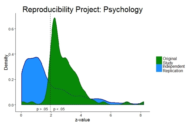
The independent replications in blue show many z-values left of the dashed line, i.e. replication attempts which were unsuccessful. Otherwise the blue distribution is relatively smooth. There is certainly nothing fishy going on around the arbitrary p = 0.05 threshold. The blue curve looks very much like what I would expect psychological research to be if questionable research practices did not exist.

However, the story is completely different for the green distribution representing the original effects. Just right of the arbitrary p = 0.05 threshold there is a surprising clustering of z-values. It’s as if the human mind magically leads to effects which are just about significant rather than just about not significant. This bump immediately to the right of the dashed line is a clear sign that original authors used questionable research practices. This behaviour renders psychological research unreplicable.

For the expert reader, the formal analysis of the caliper test is shown in the table below using both a Bayesian analysis and a classical frequentist analysis. The conclusion is clear. There is no strong evidence for replication studies failing the caliper test, indicating that questionable research practices were probably not employed. The original studies do not pass the caliper test, indicating that questionable research practices were employed.

 

	over caliper (significant)	below caliper (non-sign.)	Binomial test	Bayesian proportion test	posterior median [95% Credible Interval]1
	10 % caliper (1.76 < z < 1.96 versus 1.96 < z < 2.16)
Original	9	4	p = 0.267	BF10 = 1.09	0.53 [-0.36; 1.55]
Replication	3	2	p = 1	BF01 = 1.30	0.18 [-1.00; 1.45]
	15 % caliper (1.67 < z < 1.96 versus 1.96 < z < 2.25)
Original	17	4	p = 0.007	BF10 = 12.9	1.07 [0.24; 2.08]
Replication	4	5	p = 1	BF01 = 1.54	-0.13 [-1.18; 0.87]
	20 % caliper (1.76 < z < 1.57 versus 1.96 < z < 2.35)
Original	29	4	p < 0.001	BF10 = 2813	1.59 [0.79; 2.58]
Replication	5	5	p = 1	BF01 = 1.64	0.00 [-0.99; 0.98]

¹Based on 100,000 draws from the posterior distribution of log odds.

 

As far as I know, this is the first analysis showing that data from the original studies of the Reproducibility Project: Psychology point to questionable research practices [I have since been made aware of others, see this comment below]. Instead of sloppy science on the part of independent replication teams, this analysis rather points to original investigators employing questionable research practices. This alone could explain the surprisingly low replication rates in psychology.

Psychology failing the caliper test is by no means a new insight. Huge text-mining analyses have shown that psychology as a whole tends to fail the caliper test (Kühberger et al., 2013, Head et al., 2015). The analysis I have presented here links this result to replicability. If a research field employs questionable research practices (as indicated by the caliper test) then it can no longer claim to deliver insights which stand the replication test (as indicated by the Reproducibility Project: Psychology).

It is time to get rid of questionable research practices. There are enough ideas for how to do so (e.g., Asendorpf et al., 2013; Ioannidis, Munafò, Fusar-Poli, Nosek, & Lakens, 2014). The Reproducibility Project: Psychology shows why there is no time to waste: it is currently very difficult to distinguish an interesting psychological effect from a statistical fluke. I doubt that this state of affairs is what psychological researchers get paid for.

PS: full R-code for recreating all analyses and figures is posted below. If you find mistakes please let me know.

PPS: I am indebted to Jelte Wicherts for pointing me to this analysis.

Update 25/4/2015:

I adjusted text to clarify that caliper test cannot distinguish between many different questionable research practices, following tweet by Daniël Lakens.

I toned down the language somewhat following tweet by Daniel Bennett.

I added reference to Uli Schimmack’s analysis by linking his comment.

— — —

Asendorpf, J., Conner, M., De Fruyt, F., De Houwer, J., Denissen, J., Fiedler, K., Fiedler, S., Funder, D., Kliegl, R., Nosek, B., Perugini, M., Roberts, B., Schmitt, M., van Aken, M., Weber, H., & Wicherts, J. (2013). Recommendations for Increasing Replicability in Psychology European Journal of Personality, 27 (2), 108-119 DOI: 10.1002/per.1919

Gerber, A., & Malhotra, N. (2008). Publication Bias in Empirical Sociological Research: Do Arbitrary Significance Levels Distort Published Results? Sociological Methods & Research, 37 (1), 3-30 DOI: 10.1177/0049124108318973

Gerber, A., Malhotra, N., Dowling, C., & Doherty, D. (2010). Publication Bias in Two Political Behavior Literatures American Politics Research, 38 (4), 591-613 DOI: 10.1177/1532673X09350979

Gilbert, D., King, G., Pettigrew, S., & Wilson, T. (2016). Comment on “Estimating the reproducibility of psychological science” Science, 351 (6277), 1037-1037 DOI: 10.1126/science.aad7243

Head ML, Holman L, Lanfear R, Kahn AT, & Jennions MD (2015). The extent and consequences of p-hacking in science. PLoS biology, 13 (3) PMID: 25768323

Ioannidis JP, Munafò MR, Fusar-Poli P, Nosek BA, & David SP (2014). Publication and other reporting biases in cognitive sciences: detection, prevalence, and prevention. Trends in cognitive sciences, 18 (5), 235-41 PMID: 24656991

Kühberger A, Fritz A, & Scherndl T (2014). Publication bias in psychology: a diagnosis based on the correlation between effect size and sample size. PloS one, 9 (9) PMID: 25192357

Kunert R (2016). Internal conceptual replications do not increase independent replication success. Psychonomic bulletin & review PMID: 27068542

Open Science Collaboration (2015). Estimating the reproducibility of psychological science Science, 349 (6251) DOI: 10.1126/science.aac4716

— — —

##################################################################################################################
# Script for article "Questionable research practices in original studies of Reproducibility Project: Psychology"#
# Submitted to Brain's Idea (status: published)                                                                                               #
# Responsible for this file: R. Kunert (rikunert@gmail.com)                                                      # 
##################################################################################################################    
 
##########################################################################################################################################################################################
#-----------------------------------------------------------------------------------------------------------------------------------------------------------------------------------------
#Figure 1: p-value density
 
# source functions
if(!require(httr)){install.packages('httr')}
library(httr)
info <- GET('https://osf.io/b2vn7/?action=download', write_disk('functions.r', overwrite = TRUE)) #downloads data file from the OSF
source('functions.r')
 
if(!require(devtools)){install.packages('devtools')} #RPP functions
library(devtools)
source_url('https://raw.githubusercontent.com/FredHasselman/toolboxR/master/C-3PR.R')
in.IT(c('ggplot2','RColorBrewer','lattice','gridExtra','plyr','dplyr','httr','extrafont'))
 
if(!require(BayesFactor)){install.packages('BayesFactor')} #Bayesian analysis
library(BayesFactor)
 
if(!require(BEST)){install.packages('BEST')} #distribution overlap
library(BEST)#requires JAGS version 3
 
if(!require(RCurl)){install.packages('RCurl')} #
library(RCurl)#
 
#the following few lines are an excerpt of the Reproducibility Project: Psychology's 
# masterscript.R to be found here: https://osf.io/vdnrb/
 
# Read in Tilburg data
info <- GET('https://osf.io/fgjvw/?action=download', write_disk('rpp_data.csv', overwrite = TRUE)) #downloads data file from the OSF
MASTER <- read.csv("rpp_data.csv")[1:167, ]
colnames(MASTER)[1] <- "ID" # Change first column name to ID to be able to load .csv file
 
#for studies with exact p-values
id <- MASTER$ID[!is.na(MASTER$T_pval_USE..O.) & !is.na(MASTER$T_pval_USE..R.)]
 
#FYI: turn p-values into z-scores 
#z = qnorm(1 - (pval/2)) 
 
#prepare data point for plotting
dat_vis <- data.frame(p = c(MASTER$T_pval_USE..O.[id],
                            MASTER$T_pval_USE..R.[id], MASTER$T_pval_USE..R.[id]),
                      z = c(qnorm(1 - (MASTER$T_pval_USE..O.[id]/2)),
                            qnorm(1 - (MASTER$T_pval_USE..R.[id]/2)),
                            qnorm(1 - (MASTER$T_pval_USE..R.[id]/2))),
                      Study_set= c(rep("Original Publications", length(id)),
                                   rep("Independent Replications", length(id)),
                                   rep("zIndependent Replications2", length(id))))
 
#prepare plotting colours etc
cols_emp_in = c("#1E90FF","#088A08")#colour_definitions of area
cols_emp_out = c("#08088a","#0B610B")#colour_definitions of outline
legend_labels = list("Independent\nReplication", "Original\nStudy")
 
#execute actual plotting
density_plot = ggplot(dat_vis, aes(x=z, fill = Study_set, color = Study_set, linetype = Study_set))+
  geom_density(adjust =0.6, size = 1, alpha=1) +  #density plot call
  scale_linetype_manual(values = c(1,1,3)) +#outline line types
  scale_fill_manual(values = c(cols_emp_in,NA), labels = legend_labels)+#specify the to be used colours (outline)
  scale_color_manual(values = cols_emp_out[c(1,2,1)])+#specify the to be used colours (area)
  labs(x="z-value", y="Density")+ #add axis titles  
  ggtitle("Reproducibility Project: Psychology") +#add title
  geom_vline(xintercept = qnorm(1 - (0.05/2)), linetype = 2) +
  annotate("text", x = 2.92, y = -0.02, label = "p < .05", vjust = 1, hjust = 1)+
  annotate("text", x = 1.8, y = -0.02, label = "p > .05", vjust = 1, hjust = 1)+
  theme(legend.position="none",#remove legend
        panel.grid.major = element_blank(),
        panel.grid.minor = element_blank(),
        panel.border = element_blank(),
        axis.line  = element_line(colour = "black"),#clean look
        text = element_text(size=18),
        plot.title=element_text(size=30))
density_plot
 
#common legend
#draw a nonsense bar graph which will provide a legend
legend_labels = list("Independent\nReplication", "Original\nStudy")
dat_vis <- data.frame(ric = factor(legend_labels, levels=legend_labels), kun = c(1, 2))
dat_vis$ric = relevel(dat_vis$ric, "Original\nStudy")
nonsense_plot = ggplot(data=dat_vis, aes(x=ric, y=kun, fill=ric)) + 
  geom_bar(stat="identity")+
  scale_fill_manual(values=cols_emp_in[c(2,1)], name=" ") +
  theme(legend.text=element_text(size=18))
#extract legend
tmp <- ggplot_gtable(ggplot_build(nonsense_plot)) 
leg <- which(sapply(tmp$grobs, function(x) x$name) == "guide-box") 
leg_plot <- tmp$grobs[[leg]]
#combine plots
grid.arrange(grobs = list(density_plot,leg_plot), ncol = 2, widths = c(2,0.4))
 
#caliper test according to Gerber et al.
 
#turn p-values into z-values
z_o = qnorm(1 - (MASTER$T_pval_USE..O.[id]/2))
z_r = qnorm(1 - (MASTER$T_pval_USE..R.[id]/2))
 
#How many draws are to be taken from posterior distribution for BF and Credible Interval calculations? The more samples the more precise the estimate and the slower the calculation.
draws = 10000 * 10#BayesFactor package standard = 10000
 
#choose one of the calipers
#z_c = c(1.76, 2.16)#10% caliper
#z_c = c(1.67, 2.25)#15% caliper
#z_c = c(1.57, 2.35)#20% caliper
 
#calculate counts
print(sprintf('Originals: over caliper N = %d', sum(z_o <= z_c[2] & z_o >= 1.96)))
print(sprintf('Originals: under caliper N = %d', sum(z_o >= z_c[1] & z_o <= 1.96)))
print(sprintf('Replications: over caliper N = %d', sum(z_r <= z_c[2] & z_r >= 1.96)))
print(sprintf('Replications: under caliper N = %d', sum(z_r >= z_c[1] & z_r <= 1.96)))
 
#formal caliper test: originals
#Bayesian analysis
bf = proportionBF(sum(z_o <= z_c[2] & z_o >= 1.96), sum(z_o >= z_c[1] & z_o <= z_c[2]), p = 1/2)
sprintf('Bayesian test of single proportion: BF10 = %1.2f', exp(bf@bayesFactor$bf))#exponentiate BF10 because stored as natural log
#sample from posterior
samples_o = proportionBF(sum(z_o <= z_c[2] & z_o >= 1.96), sum(z_o >= z_c[1] & z_o <= z_c[2]), p = 1/2,
                       posterior = TRUE, iterations = draws)
plot(samples_o[,"logodds"])
sprintf('Posterior Median = %1.2f [%1.2f; %1.2f]',
        median(samples_o[,"logodds"]),#Median 
        quantile(samples_o[,"logodds"], 0.025),#Lower edge of 95% Credible Interval
        quantile(samples_o[,"logodds"], 0.975))#Higher edge of 95% Credible Interval
#classical frequentist test
bt = binom.test(sum(z_o <= z_c[2] & z_o >= 1.96), sum(z_o >= z_c[1] & z_o <= z_c[2]), p = 1/2)
sprintf('Binomial test: p = %1.3f', bt$p.value)#
 
#formal caliper test: replications
bf = proportionBF(sum(z_r <= z_c[2] & z_r >= 1.96), sum(z_r >= z_c[1] & z_r <= z_c[2]), p = 1/2)
sprintf('Bayesian test of single proportion: BF01 = %1.2f', 1/exp(bf@bayesFactor$bf))#exponentiate BF10 because stored as natural log, turn into BF01
#sample from posterior
samples_r = proportionBF(sum(z_r <= z_c[2] & z_r >= 1.96), sum(z_r >= z_c[1] & z_r <= z_c[2]), p = 1/2,
                       posterior = TRUE, iterations = draws)
plot(samples[,"logodds"])
sprintf('Posterior Median = %1.2f [%1.2f; %1.2f]',
        median(samples_r[,"logodds"]),#Median 
        quantile(samples_r[,"logodds"], 0.025),#Lower edge of 95% Credible Interval
        quantile(samples_r[,"logodds"], 0.975))#Higher edge of 95% Credible Interval
#classical frequentist test
bt = binom.test(sum(z_r <= z_c[2] & z_r >= 1.96), sum(z_r >= z_c[1] & z_r <= z_c[2]), p = 1/2)
sprintf('Binomial test: p = %1.3f', bt$p.value)#
 
#possibly of interest: overlap of posteriors
#postPriorOverlap(samples_o[,"logodds"], samples_r[,"logodds"])#overlap of distribitions

Created by Pretty R at inside-R.org