A critical comment on “Contextual sensitivity in scientific reproducibility”

Psychological science is surprisingly difficult to replicate (Open Science Collaboration, 2015). Researchers are desperate to find out why. A new study in the prestigious journal PNAS (Van Bavel et al., 2016) claims that unknown contextual factors of psychological phenomena (“hidden moderators”) are to blame. The more an effect is sensitive to unknown contextual factors, the less likely a successful replication is. In this blog post I will lay out why I am not convinced by this argument.

Before I start I should say that I really appreciate that the authors of this paper make their point with reference to data and analyses thereof. I believe that this is a big improvement on the state of the replicability debate of a few years back when it was dominated by less substantiated opinions. Moreover, they share their key data and some analysis code, following good scientific practice. Still, I am not convinced by their argument. Here’s why:

1) No full engagement with the opposite side of the argument

Van Bavel et al.’s (2016) suggested influence of replication contexts on replication success cannot explain the following patterns in the data set they used (Open Science Collaboration, 2015):

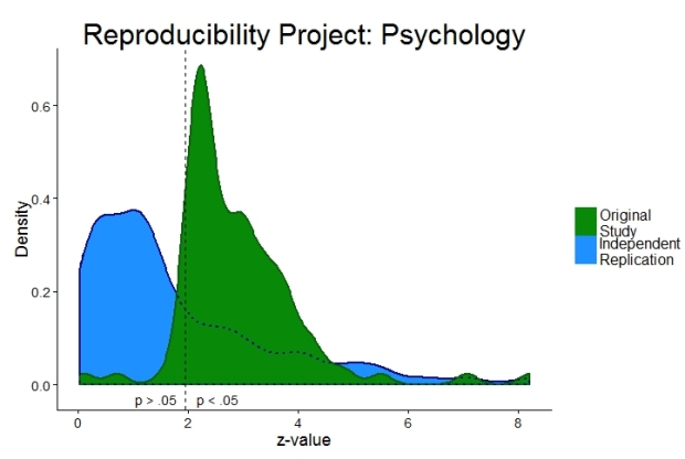
a) replication effect sizes are mostly lower than original effect sizes. Effects might well “vary by [replication] context” (p. 2) but why the consistent reduction in effect size when replicating an effect?

b) internal conceptual replications are not related to independent replication success (Kunert, 2016). This goes directly against Van Bavel et al.’s (2016) suggestion that “conceptual replications can even improve the probability of successful replications” (p. 5).

c) why are most original effects just barely statistically significant (see previous blog post)?

I believe that all three patterns point to some combination of questionable research practices affecting the original studies. Nothing in Van Bavel et al.’s (2016) article manages to convince me otherwise.

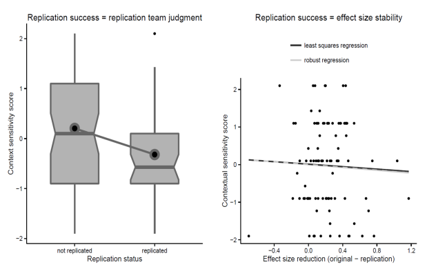
2) The central result completely depends on how you define ‘replication success’

The central claim of the article is based on the correlation between one measure of replication success (subjective judgment by replication team of whether replication was successful) and one measure of the contextual sensitivity of a replicated effect. While the strength of the association (r = -.23) is statistically significant (p = .024), it doesn’t actually provide convincing evidence for either the null or the alternative hypothesis according to a standard Bayesian JZS correlation test (BF₀₁ = 1). [For all analyses: R-code below.]

Moreover, another measure of replication success (reduction of effect size between original and replication study) is so weakly correlated with the contextual sensitivity variable (r = -.01) as to provide strong evidence for a lack of association between contextual sensitivity and replication success (BF₀₁ = 12, notice that even the direction of the correlation is in the wrong direction according to Van Bavel et al.’s (2016) account).

[Update: The corresponding values for the other measures of replication success are: replication p < .05 (r = -0.18; p = .0721; BF₀₁ = 2.5), original effect size in 95%CI of replication effect size (r = -.3, p = .0032, BF₁₀ = 6). I could not locate the data column for whether the meta-analytic effect size is different from zero.]

3) The contextual sensitivity variable could be confounded

How do we know which original effects were plagued by hidden moderators (i.e. by unknown context sensitivity) if, well, these moderators are hidden? Three of the authors of the article simply rated all replicated studies for contextual sensitivity without knowing each study’s replication status (but after the replication success of each study was known in general). The authors provide evidence for the ratings to be reliable but no one knows whether they are valid.

For example, the raters tried not to be influenced by ‘whether the specific replication attempt in question would succeed’ (p. 2). Still, all raters knew they would benefit (in the form of a prestigious publication) from a significant association between their ratings and replication success. How do we know that the ratings do not simply reflect some sort of implicit replicability doubt? From another PNAS study (Dreber et al., 2015) we know that scientists can predict replication success before a replication study is run.

Revealing hidden moderators

My problem with the contextual sensitivity account claiming that unknown moderators are to blame for replication failures is not so much that it is an unlikely explanation. I agree with Van Bavel et al. (2016) that some psychological phenomena are more sensitive to replication contexts than others. I would equally welcome it if scientific authors were more cautious in generalising their results.

My problem is that this account is so general as to be nearly unfalsifiable, and an unfalsifiable account is scientifically useless. Somehow unknown moderators always get invoked once a replication attempt has failed. All sorts of wild claims could be retrospectively claimed to be true within the context of the original finding.

In short: a convincing claim that contextual factors are to blame for replication failures needs to reveal the crucial replication contexts and then show that they indeed influence replication success. The proof of the unknown pudding is in the eating.

— — —
Dreber, A., Pfeiffer, T., Almenberg, J., Isaksson, S., Wilson, B., Chen, Y., Nosek, B., & Johannesson, M. (2015). Using prediction markets to estimate the reproducibility of scientific research Proceedings of the National Academy of Sciences, 112 (50), 15343-15347 DOI: 10.1073/pnas.1516179112

Kunert, R. (2016). Internal conceptual replications do not increase independent replication success Psychonomic Bulletin & Review DOI: 10.3758/s13423-016-1030-9

Open Science Collaboration (2015). Estimating the reproducibility of psychological science Science, 349 (6251) DOI: 10.1126/science.aac4716

Van Bavel, J.J., Mende-Siedlecki, P., Brady, W.J., & Reinero, D.A. (2016). Contextual sensitivity in scientific reproducibility PNAS
— — —

########################################################################################################
# Script for article "A critical comment on "Contextual sensitivity in scientific reproducibility""    #
# Submitted to Brain's Idea                                                                            #
# Responsible for this file: R. Kunert (rikunert@gmail.com)                                            # 
########################################################################################################   
 
# source functions
if(!require(devtools)){install.packages('devtools')} #RPP functions
library(devtools)
source_url('https://raw.githubusercontent.com/FredHasselman/toolboxR/master/C-3PR.R')
in.IT(c('ggplot2','RColorBrewer','lattice','gridExtra','plyr','dplyr','httr','extrafont'))
 
if(!require(BayesMed)){install.packages('BayesMed')} #Bayesian analysis of correlation
library(BayesMed)
 
if(!require(Hmisc)){install.packages('Hmisc')} #correlations
library(Hmisc)
 
if(!require(reshape2)){install.packages('reshape2')}#melt function
library(reshape2)
 
if(!require(grid)){install.packages('grid')} #arranging figures
library(grid)
 
#get raw data from OSF website
info <- GET('https://osf.io/pra2u/?action=download', write_disk('rpp_Bevel_data.csv', overwrite = TRUE)) #downloads data file from the OSF
RPPdata <- read.csv("rpp_Bevel_data.csv")[1:100, ]
colnames(RPPdata)[1] <- "ID" # Change first column name
 
#------------------------------------------------------------------------------------------------------------
#2) The central result completely depends on how you define 'replication success'----------------------------
 
#replication with subjective judgment of whether it replicated
rcorr(RPPdata$ContextVariable_C, RPPdata$Replicate_Binary, type = 'spearman')
#As far as I know there is currently no Bayesian Spearman rank correlation analysis. Therefore, use standard correlation analysis with raw and ranked data and hope that the result is similar.
#parametric Bayes factor test
bf = jzs_cor(RPPdata$ContextVariable_C, RPPdata$Replicate_Binary)#parametric Bayes factor test
plot(bf$alpha_samples)
1/bf$BayesFactor#BF01 provides support for null hypothesis over alternative
#parametric Bayes factor test with ranked data
bf = jzs_cor(rank(RPPdata$ContextVariable_C), rank(RPPdata$Replicate_Binary))#parametric Bayes factor test
plot(bf$alpha_samples)
1/bf$BayesFactor#BF01 provides support for null hypothesis over alternative
 
#replication with effect size reduction
rcorr(RPPdata$ContextVariable_C[!is.na(RPPdata$FXSize_Diff)], RPPdata$FXSize_Diff[!is.na(RPPdata$FXSize_Diff)], type = 'spearman')
#parametric Bayes factor test
bf = jzs_cor(RPPdata$ContextVariable_C[!is.na(RPPdata$FXSize_Diff)], RPPdata$FXSize_Diff[!is.na(RPPdata$FXSize_Diff)])
plot(bf$alpha_samples)
1/bf$BayesFactor#BF01 provides support for null hypothesis over alternative
#parametric Bayes factor test with ranked data
bf = jzs_cor(rank(RPPdata$ContextVariable_C[!is.na(RPPdata$FXSize_Diff)]), rank(RPPdata$FXSize_Diff[!is.na(RPPdata$FXSize_Diff)]))
plot(bf$alpha_samples)
1/bf$BayesFactor#BF01 provides support for null hypothesis over alternative
 
#------------------------------------------------------------------------------------------------------------
#Figure 1----------------------------------------------------------------------------------------------------
 
#general look
theme_set(theme_bw(12)+#remove gray background, set font-size
            theme(axis.line = element_line(colour = "black"),
                  panel.grid.major = element_blank(),
                  panel.grid.minor = element_blank(),
                  panel.background = element_blank(),
                  panel.border = element_blank(),
                  legend.title = element_blank(),
                  legend.key = element_blank(),
                  legend.position = "top",
                  legend.direction = 'vertical'))
 
#Panel A: replication success measure = binary replication team judgment
dat_box = melt(data.frame(dat = c(RPPdata$ContextVariable_C[RPPdata$Replicate_Binary == 1],
                                  RPPdata$ContextVariable_C[RPPdata$Replicate_Binary == 0]),
                          replication_status = c(rep('replicated', sum(RPPdata$Replicate_Binary == 1)),
                                                 rep('not replicated', sum(RPPdata$Replicate_Binary == 0)))),
               id = c('replication_status'))
 
#draw basic box plot
plot_box = ggplot(dat_box, aes(x=replication_status, y=value)) +
  geom_boxplot(size = 1.2,#line size
               alpha = 0.3,#transparency of fill colour
               width = 0.8,#box width
               notch = T, notchwidth = 0.8,#notch setting               
               show_guide = F,#do not show legend
               fill='black', color='grey40') +  
  labs(x = "Replication status", y = "Context sensitivity score")#axis titles
 
#add mean values and rhythm effect lines to box plot
 
#prepare data frame
dat_sum = melt(data.frame(dat = c(mean(RPPdata$ContextVariable_C[RPPdata$Replicate_Binary == 1]),
                                  mean(RPPdata$ContextVariable_C[RPPdata$Replicate_Binary == 0])),
                          replication_status = c('replicated', 'not replicated')),
               id = 'replication_status')
 
#add mean values
plot_box = plot_box +
  geom_line(data = dat_sum, mapping = aes(y = value, group = 1),
            size= c(1.5), color = 'grey40')+
  geom_point(data = dat_sum, size=12, shape=20,#dot rim
             fill = 'grey40',
             color = 'grey40') +
  geom_point(data = dat_sum, size=6, shape=20,#dot fill
             fill = 'black',
             color = 'black')
plot_box
 
#Panel B: replication success measure = effect size reduction
dat_corr = data.frame("x" = RPPdata$FXSize_Diff[!is.na(RPPdata$FXSize_Diff)],
                      "y" = RPPdata$ContextVariable_C[!is.na(RPPdata$FXSize_Diff)])#plotted data
 
plot_corr = ggplot(dat_corr, aes(x = x, y = y))+
  geom_point(size = 2) +#add points
  stat_smooth(method = "lm", size = 1, se = FALSE,
              aes(colour = "least squares regression")) +
  stat_smooth(method = "rlm", size = 1, se = FALSE,
              aes(colour = "robust regression")) +
  labs(x = "Effect size reduction (original - replication)", y = "Contextual sensitivity score") +#axis labels
  scale_color_grey()+#colour scale for lines
  stat_smooth(method = "lm", size = 1, se = FALSE,
              aes(colour = "least squares regression"),
              lty = 2)
plot_corr
 
#arrange figure with both panels
multi.PLOT(plot_box + ggtitle("Replication success = replication team judgment"),
           plot_corr + ggtitle("Replication success = effect size stability"),
           cols=2)

Created by Pretty R at inside-R.org

Yet more evidence for questionable research practices in original studies of Reproducibility Project: Psychology

The replicability of psychological research is surprisingly low. Why? In this blog post I present new evidence showing that questionable research practices contributed to failures to replicate psychological effects.

Quick recap. A recent publication in Science claims that only around 40% of psychological findings are replicable, based on 100 replication attempts in the Reproducibility Project Psychology (Open Science Collaboration, 2015). A few months later, a critical commentary in the same journal made all sorts of claims, including that the surprisingly low 40% replication success rate is due to replications having been unfaithful to the original studies’ methods (Gilbert et al., 2016). A little while later, I published an article in Psychonomic Bulletin & Review re-analysing the data by the 100 replication teams (Kunert, 2016). I found evidence for questionable research practices being at the heart of failures to replicate, rather than the unfaithfulness of replications to original methods.

However, my previous re-analysis depended on replication teams having done good work. In this blog post I will show that even when just looking at the original studies in the Reproducibility Project: Psychology one cannot fail to notice that questionable research practices were employed by the original discoverers of the effects which often failed to replicate. The reanalysis I will present here is based on the caliper test introduced by Gerber and colleagues (Gerber & Malhotra, 2008; Gerber et al., 2010).

The idea of the caliper test is simple. The research community has decided that an entirely arbitrary threshold of p = 0.05 distinguishes between effects which might just be due to chance (p > 0.05) and effects which are more likely due to something other than chance (p < 0.05). If researchers want to game the system they slightly rig their methods and analyses to push their p-values just below the arbitrary border between ‘statistical fluke’ and ‘interesting effect’. Alternatively, they just don’t publish anything which came up p > 0.05. Such behaviour should lead to an unlikely amount of p-values just below 0.05 compared to just above 0.05.

The figure below shows the data of the Reproducibility Project: Psychology. On the horizontal axis I plot z-values which are related to p-values. The higher the z-value the lower the p-value. On the vertical axis I just show how many z-values I found in each range. The dashed vertical line is the arbitrary threshold between p < .05 (significant effects on the right) and p > .05 (non-significant effects on the left).

The independent replications in blue show many z-values left of the dashed line, i.e. replication attempts which were unsuccessful. Otherwise the blue distribution is relatively smooth. There is certainly nothing fishy going on around the arbitrary p = 0.05 threshold. The blue curve looks very much like what I would expect psychological research to be if questionable research practices did not exist.

However, the story is completely different for the green distribution representing the original effects. Just right of the arbitrary p = 0.05 threshold there is a surprising clustering of z-values. It’s as if the human mind magically leads to effects which are just about significant rather than just about not significant. This bump immediately to the right of the dashed line is a clear sign that original authors used questionable research practices. This behaviour renders psychological research unreplicable.

For the expert reader, the formal analysis of the caliper test is shown in the table below using both a Bayesian analysis and a classical frequentist analysis. The conclusion is clear. There is no strong evidence for replication studies failing the caliper test, indicating that questionable research practices were probably not employed. The original studies do not pass the caliper test, indicating that questionable research practices were employed.

 

	over caliper (significant)	below caliper (non-sign.)	Binomial test	Bayesian proportion test	posterior median [95% Credible Interval]1
	10 % caliper (1.76 < z < 1.96 versus 1.96 < z < 2.16)
Original	9	4	p = 0.267	BF10 = 1.09	0.53 [-0.36; 1.55]
Replication	3	2	p = 1	BF01 = 1.30	0.18 [-1.00; 1.45]
	15 % caliper (1.67 < z < 1.96 versus 1.96 < z < 2.25)
Original	17	4	p = 0.007	BF10 = 12.9	1.07 [0.24; 2.08]
Replication	4	5	p = 1	BF01 = 1.54	-0.13 [-1.18; 0.87]
	20 % caliper (1.76 < z < 1.57 versus 1.96 < z < 2.35)
Original	29	4	p < 0.001	BF10 = 2813	1.59 [0.79; 2.58]
Replication	5	5	p = 1	BF01 = 1.64	0.00 [-0.99; 0.98]

¹Based on 100,000 draws from the posterior distribution of log odds.

 

As far as I know, this is the first analysis showing that data from the original studies of the Reproducibility Project: Psychology point to questionable research practices [I have since been made aware of others, see this comment below]. Instead of sloppy science on the part of independent replication teams, this analysis rather points to original investigators employing questionable research practices. This alone could explain the surprisingly low replication rates in psychology.

Psychology failing the caliper test is by no means a new insight. Huge text-mining analyses have shown that psychology as a whole tends to fail the caliper test (Kühberger et al., 2013, Head et al., 2015). The analysis I have presented here links this result to replicability. If a research field employs questionable research practices (as indicated by the caliper test) then it can no longer claim to deliver insights which stand the replication test (as indicated by the Reproducibility Project: Psychology).

It is time to get rid of questionable research practices. There are enough ideas for how to do so (e.g., Asendorpf et al., 2013; Ioannidis, Munafò, Fusar-Poli, Nosek, & Lakens, 2014). The Reproducibility Project: Psychology shows why there is no time to waste: it is currently very difficult to distinguish an interesting psychological effect from a statistical fluke. I doubt that this state of affairs is what psychological researchers get paid for.

PS: full R-code for recreating all analyses and figures is posted below. If you find mistakes please let me know.

PPS: I am indebted to Jelte Wicherts for pointing me to this analysis.

Update 25/4/2015:

I adjusted text to clarify that caliper test cannot distinguish between many different questionable research practices, following tweet by Daniël Lakens.

I toned down the language somewhat following tweet by Daniel Bennett.

I added reference to Uli Schimmack’s analysis by linking his comment.

— — —

Asendorpf, J., Conner, M., De Fruyt, F., De Houwer, J., Denissen, J., Fiedler, K., Fiedler, S., Funder, D., Kliegl, R., Nosek, B., Perugini, M., Roberts, B., Schmitt, M., van Aken, M., Weber, H., & Wicherts, J. (2013). Recommendations for Increasing Replicability in Psychology European Journal of Personality, 27 (2), 108-119 DOI: 10.1002/per.1919

Gerber, A., & Malhotra, N. (2008). Publication Bias in Empirical Sociological Research: Do Arbitrary Significance Levels Distort Published Results? Sociological Methods & Research, 37 (1), 3-30 DOI: 10.1177/0049124108318973

Gerber, A., Malhotra, N., Dowling, C., & Doherty, D. (2010). Publication Bias in Two Political Behavior Literatures American Politics Research, 38 (4), 591-613 DOI: 10.1177/1532673X09350979

Gilbert, D., King, G., Pettigrew, S., & Wilson, T. (2016). Comment on “Estimating the reproducibility of psychological science” Science, 351 (6277), 1037-1037 DOI: 10.1126/science.aad7243

Head ML, Holman L, Lanfear R, Kahn AT, & Jennions MD (2015). The extent and consequences of p-hacking in science. PLoS biology, 13 (3) PMID: 25768323

Ioannidis JP, Munafò MR, Fusar-Poli P, Nosek BA, & David SP (2014). Publication and other reporting biases in cognitive sciences: detection, prevalence, and prevention. Trends in cognitive sciences, 18 (5), 235-41 PMID: 24656991

Kühberger A, Fritz A, & Scherndl T (2014). Publication bias in psychology: a diagnosis based on the correlation between effect size and sample size. PloS one, 9 (9) PMID: 25192357

Kunert R (2016). Internal conceptual replications do not increase independent replication success. Psychonomic bulletin & review PMID: 27068542

Open Science Collaboration (2015). Estimating the reproducibility of psychological science Science, 349 (6251) DOI: 10.1126/science.aac4716

— — —

##################################################################################################################
# Script for article "Questionable research practices in original studies of Reproducibility Project: Psychology"#
# Submitted to Brain's Idea (status: published)                                                                                               #
# Responsible for this file: R. Kunert (rikunert@gmail.com)                                                      # 
##################################################################################################################    
 
##########################################################################################################################################################################################
#-----------------------------------------------------------------------------------------------------------------------------------------------------------------------------------------
#Figure 1: p-value density
 
# source functions
if(!require(httr)){install.packages('httr')}
library(httr)
info <- GET('https://osf.io/b2vn7/?action=download', write_disk('functions.r', overwrite = TRUE)) #downloads data file from the OSF
source('functions.r')
 
if(!require(devtools)){install.packages('devtools')} #RPP functions
library(devtools)
source_url('https://raw.githubusercontent.com/FredHasselman/toolboxR/master/C-3PR.R')
in.IT(c('ggplot2','RColorBrewer','lattice','gridExtra','plyr','dplyr','httr','extrafont'))
 
if(!require(BayesFactor)){install.packages('BayesFactor')} #Bayesian analysis
library(BayesFactor)
 
if(!require(BEST)){install.packages('BEST')} #distribution overlap
library(BEST)#requires JAGS version 3
 
if(!require(RCurl)){install.packages('RCurl')} #
library(RCurl)#
 
#the following few lines are an excerpt of the Reproducibility Project: Psychology's 
# masterscript.R to be found here: https://osf.io/vdnrb/
 
# Read in Tilburg data
info <- GET('https://osf.io/fgjvw/?action=download', write_disk('rpp_data.csv', overwrite = TRUE)) #downloads data file from the OSF
MASTER <- read.csv("rpp_data.csv")[1:167, ]
colnames(MASTER)[1] <- "ID" # Change first column name to ID to be able to load .csv file
 
#for studies with exact p-values
id <- MASTER$ID[!is.na(MASTER$T_pval_USE..O.) & !is.na(MASTER$T_pval_USE..R.)]
 
#FYI: turn p-values into z-scores 
#z = qnorm(1 - (pval/2)) 
 
#prepare data point for plotting
dat_vis <- data.frame(p = c(MASTER$T_pval_USE..O.[id],
                            MASTER$T_pval_USE..R.[id], MASTER$T_pval_USE..R.[id]),
                      z = c(qnorm(1 - (MASTER$T_pval_USE..O.[id]/2)),
                            qnorm(1 - (MASTER$T_pval_USE..R.[id]/2)),
                            qnorm(1 - (MASTER$T_pval_USE..R.[id]/2))),
                      Study_set= c(rep("Original Publications", length(id)),
                                   rep("Independent Replications", length(id)),
                                   rep("zIndependent Replications2", length(id))))
 
#prepare plotting colours etc
cols_emp_in = c("#1E90FF","#088A08")#colour_definitions of area
cols_emp_out = c("#08088a","#0B610B")#colour_definitions of outline
legend_labels = list("Independent\nReplication", "Original\nStudy")
 
#execute actual plotting
density_plot = ggplot(dat_vis, aes(x=z, fill = Study_set, color = Study_set, linetype = Study_set))+
  geom_density(adjust =0.6, size = 1, alpha=1) +  #density plot call
  scale_linetype_manual(values = c(1,1,3)) +#outline line types
  scale_fill_manual(values = c(cols_emp_in,NA), labels = legend_labels)+#specify the to be used colours (outline)
  scale_color_manual(values = cols_emp_out[c(1,2,1)])+#specify the to be used colours (area)
  labs(x="z-value", y="Density")+ #add axis titles  
  ggtitle("Reproducibility Project: Psychology") +#add title
  geom_vline(xintercept = qnorm(1 - (0.05/2)), linetype = 2) +
  annotate("text", x = 2.92, y = -0.02, label = "p < .05", vjust = 1, hjust = 1)+
  annotate("text", x = 1.8, y = -0.02, label = "p > .05", vjust = 1, hjust = 1)+
  theme(legend.position="none",#remove legend
        panel.grid.major = element_blank(),
        panel.grid.minor = element_blank(),
        panel.border = element_blank(),
        axis.line  = element_line(colour = "black"),#clean look
        text = element_text(size=18),
        plot.title=element_text(size=30))
density_plot
 
#common legend
#draw a nonsense bar graph which will provide a legend
legend_labels = list("Independent\nReplication", "Original\nStudy")
dat_vis <- data.frame(ric = factor(legend_labels, levels=legend_labels), kun = c(1, 2))
dat_vis$ric = relevel(dat_vis$ric, "Original\nStudy")
nonsense_plot = ggplot(data=dat_vis, aes(x=ric, y=kun, fill=ric)) + 
  geom_bar(stat="identity")+
  scale_fill_manual(values=cols_emp_in[c(2,1)], name=" ") +
  theme(legend.text=element_text(size=18))
#extract legend
tmp <- ggplot_gtable(ggplot_build(nonsense_plot)) 
leg <- which(sapply(tmp$grobs, function(x) x$name) == "guide-box") 
leg_plot <- tmp$grobs[[leg]]
#combine plots
grid.arrange(grobs = list(density_plot,leg_plot), ncol = 2, widths = c(2,0.4))
 
#caliper test according to Gerber et al.
 
#turn p-values into z-values
z_o = qnorm(1 - (MASTER$T_pval_USE..O.[id]/2))
z_r = qnorm(1 - (MASTER$T_pval_USE..R.[id]/2))
 
#How many draws are to be taken from posterior distribution for BF and Credible Interval calculations? The more samples the more precise the estimate and the slower the calculation.
draws = 10000 * 10#BayesFactor package standard = 10000
 
#choose one of the calipers
#z_c = c(1.76, 2.16)#10% caliper
#z_c = c(1.67, 2.25)#15% caliper
#z_c = c(1.57, 2.35)#20% caliper
 
#calculate counts
print(sprintf('Originals: over caliper N = %d', sum(z_o <= z_c[2] & z_o >= 1.96)))
print(sprintf('Originals: under caliper N = %d', sum(z_o >= z_c[1] & z_o <= 1.96)))
print(sprintf('Replications: over caliper N = %d', sum(z_r <= z_c[2] & z_r >= 1.96)))
print(sprintf('Replications: under caliper N = %d', sum(z_r >= z_c[1] & z_r <= 1.96)))
 
#formal caliper test: originals
#Bayesian analysis
bf = proportionBF(sum(z_o <= z_c[2] & z_o >= 1.96), sum(z_o >= z_c[1] & z_o <= z_c[2]), p = 1/2)
sprintf('Bayesian test of single proportion: BF10 = %1.2f', exp(bf@bayesFactor$bf))#exponentiate BF10 because stored as natural log
#sample from posterior
samples_o = proportionBF(sum(z_o <= z_c[2] & z_o >= 1.96), sum(z_o >= z_c[1] & z_o <= z_c[2]), p = 1/2,
                       posterior = TRUE, iterations = draws)
plot(samples_o[,"logodds"])
sprintf('Posterior Median = %1.2f [%1.2f; %1.2f]',
        median(samples_o[,"logodds"]),#Median 
        quantile(samples_o[,"logodds"], 0.025),#Lower edge of 95% Credible Interval
        quantile(samples_o[,"logodds"], 0.975))#Higher edge of 95% Credible Interval
#classical frequentist test
bt = binom.test(sum(z_o <= z_c[2] & z_o >= 1.96), sum(z_o >= z_c[1] & z_o <= z_c[2]), p = 1/2)
sprintf('Binomial test: p = %1.3f', bt$p.value)#
 
#formal caliper test: replications
bf = proportionBF(sum(z_r <= z_c[2] & z_r >= 1.96), sum(z_r >= z_c[1] & z_r <= z_c[2]), p = 1/2)
sprintf('Bayesian test of single proportion: BF01 = %1.2f', 1/exp(bf@bayesFactor$bf))#exponentiate BF10 because stored as natural log, turn into BF01
#sample from posterior
samples_r = proportionBF(sum(z_r <= z_c[2] & z_r >= 1.96), sum(z_r >= z_c[1] & z_r <= z_c[2]), p = 1/2,
                       posterior = TRUE, iterations = draws)
plot(samples[,"logodds"])
sprintf('Posterior Median = %1.2f [%1.2f; %1.2f]',
        median(samples_r[,"logodds"]),#Median 
        quantile(samples_r[,"logodds"], 0.025),#Lower edge of 95% Credible Interval
        quantile(samples_r[,"logodds"], 0.975))#Higher edge of 95% Credible Interval
#classical frequentist test
bt = binom.test(sum(z_r <= z_c[2] & z_r >= 1.96), sum(z_r >= z_c[1] & z_r <= z_c[2]), p = 1/2)
sprintf('Binomial test: p = %1.3f', bt$p.value)#
 
#possibly of interest: overlap of posteriors
#postPriorOverlap(samples_o[,"logodds"], samples_r[,"logodds"])#overlap of distribitions

Created by Pretty R at inside-R.org

Why are Psychological findings mostly unreplicable?

Take 97 psychological effects from top journals which are claimed to be robust. How many will replicate? Brian Nosek and his huge team tried it out and the results were sobering, to say the least. How did we get here? The data give some clues.

Sometimes the title of a paper just sounds incredible. Estimating the reproducibility of psychological science. No one had ever systematically, empirically investigated this for any science. Doing so would require huge resources. The countless authors on this paper which appeared in Science last week went to great lengths to try anyway and their findings are worrying.

When they tried to replicate 97 statistically significant effects with 92% power (i.e. a nominal 92% chance of finding the effect should it exist as claimed by the original discoverers), 89 statistically significant effect should pop up. Only 35 did. Why weren’t 54 more studies replicated?

The team behind this article also produced 95% Confidence Intervals of the replication study effect sizes. Despite their name, only 83% of them should contain the original effect size (see here why). Only 47% actually did. Why were most effect sizes much smaller in the replication?

One reason for poor replication: sampling until significant

I believe much has to do with so-called questionable research practices which I blogged about before. The consequences of this are directly visible in the openly available data of this paper. Specifically, I am focussing on the widespread practice of sampling more participants until a test result is statistically desirable, i.e. until you get a p-value below the arbitrary threshold of 0.05. The consequence is this:

Focus on the left panel first. The green replication studies show a moderate relation between the effect size they found and their pre-determined sample size. This is to be expected as the replicators wanted to be sure that they had sufficient statistical power to find their effects. Expecting small effects (lower on vertical axis) makes you plan in more participants (further right on horizontal axis). The replicators simply sampled their pre-determined number, and then analysed the data. Apparently, such a practice leads to a moderate correlation between measured effect size and sample size because what the measured effect size will be is uncertain when you start sampling.

The red original studies show a stronger relation between the effect size they found and their sample size. They must have done more than just smart a priori power calculations. I believe that they sampled until their effect was statistically significant, going back and forth between sampling and analysing their data. If, by chance, the first few participants showed the desired effect quite strongly, experimenters were happy with overestimating their effect size and stopped early. These would be red data values in the top left of the graph. If, on the other hand, the first few participants gave equivocal results, the experimenters continued for as long as necessary. Notice how this approach links sample size to the effect size measured in the experiment, hence the strong statistical relation. The approach by the replicators links the sample size merely to the expected effect size estimated before the experiment, hence the weaker association with the actually measured effect size.

The right panel shows a Bayesian correlation analysis of the data. What you are looking at is the belief in the strength of the correlation, called the posterior distribution. The overlap of the distributions can be used as a measure of believing that the correlations are not different. The overlap is less than 7%. If you are more inclined to believe in frequentist statistics, the associated p-value is .001 (Pearson and Filon’s z = 3.355). Therefore, there is strong evidence that original studies display a stronger negative correlation between sample size and measured effect size than replication studies.

The approach which – I believe – has been followed by the original research teams should be accompanied by adjustments of the p-value (see Lakens, 2014 for how to do this). If not, you misrepresent your stats and lower the chances of replication, as shown in simulation studies (Simmons et al., 2011). It is estimated that 70% of psychological researchers have sampled until their result was statistically significant without correcting their results for this (John et al., 2012). This might very well be one of the reasons why replication rates in Psychology are far lower than what they should be.

So, one approach to boosting replication rates might be to do what we claim to do anyways and what the replication studies have actually done: aquiring data first, analysing it second. Alternatively, be open about what you did and correct your results appropriately. Otherwise, you might publish nothing more than a fluke finding with no basis.

[24/10/2015: Added Bayesian analysis and changed figure. Code below is from old figure.]

[27/11/2015: Adjusted percentage overlap of posterior distributions.]

— — —
John LK, Loewenstein G, & Prelec D (2012). Measuring the prevalence of questionable research practices with incentives for truth telling. Psychological science, 23 (5), 524-32 PMID: 22508865

Lakens, D. (2014). Performing high-powered studies efficiently with sequential analyses European Journal of Social Psychology, 44 (7), 701-710 DOI: 10.1002/ejsp.2023

Open Science Collaboration (2015). Estimating the reproducibility of psychological science. Science (New York, N.Y.), 349 (6251) PMID: 26315443

Simmons, J., Nelson, L., & Simonsohn, U. (2011). False-Positive Psychology: Undisclosed Flexibility in Data Collection and Analysis Allows Presenting Anything as Significant Psychological Science, 22 (11), 1359-1366 DOI: 10.1177/0956797611417632

— — —

code for reproducing the figure (if you find mistakes, please tell me!):

## Estimating the association between sample size and effect size from data provided by the reproducibility project https://osf.io/vdnrb/

#Richard Kunert for Brain's Idea 3/9/2015
#load necessary libraries
library(httr)
library(Hmisc)
library(ggplot2)
library(cocor)

#get raw data from OSF website
info <- GET('https://osf.io/fgjvw/?action=download', write_disk('rpp_data.csv', overwrite = TRUE)) #downloads data file from the OSF
MASTER <- read.csv("rpp_data.csv")[1:167, ]
colnames(MASTER)[1] <- "ID" # Change first column name to ID to be able to load .csv file

#restrict studies to those with appropriate data
studies<-MASTER$ID[!is.na(MASTER$T_r..O.) & !is.na(MASTER$T_r..R.)] ##to keep track of which studies are which
studies<-studies[-31]##remove one problem study with absurdly high sample size (N = 23,0047)

#set font size for plotting
theme_set(theme_gray(base_size = 30))

#prepare correlation coefficients
dat_rank <- data.frame(sample_size_O = rank(cbind(MASTER$T_N_O_for_tables[studies])),
sample_size_R = rank(cbind(MASTER$T_N_R_for_tables[studies])),
effect_size_O = rank(cbind(MASTER$T_r..O.[studies])),
effect_size_R = rank(cbind(MASTER$T_r..R.[studies])))
corr_O_Spearm = rcorr(dat_rank$effect_size_O, dat_rank$sample_size_O, type = "spearman")#yes, I know the type specification is superfluous
corr_R_Spearm = rcorr(dat_rank$effect_size_R, dat$sample_size_R, type = "spearman")

#compare Spearman correlation coefficients using cocor (data needs to be ranked in order to produce Spearman correlations!)
htest = cocor(formula=~sample_size_O + effect_size_O | sample_size_R + effect_size_R,
data = dat_rank, return.htest = FALSE)

#visualisation
#prepare data frame
dat_vis <- data.frame(study = rep(c("Original", "Replication"), each=length(studies)),
sample_size = rbind(cbind(MASTER$T_N_O_for_tables[studies]), cbind(MASTER$T_N_R_for_tables[studies])),
effect_size = rbind(cbind(MASTER$T_r..O.[studies]), cbind(MASTER$T_r..R.[studies])))

#The plotting call
plot.new
ggplot(data=dat_vis, aes(x=sample_size, y=effect_size, group=study)) +#the basic scatter plot
geom_point(aes(color=study),shape=1,size=4) +#specify marker size and shape
scale_colour_hue(l=50) + # Use a slightly darker palette than normal
geom_smooth(method=lm,   # Add linear regression lines
se=FALSE,    # Don't add shaded confidence region
size=2,
aes(color=study))+#colour lines according to data points for consistency
geom_text(aes(x=750, y=0.46,
label=sprintf("Spearman rho = %1.3f (p = %1.3f)",
corr_O_Spearm$r[1,2], corr_O_Spearm$P[1,2]),
color="Original", hjust=0)) +#add text about Spearman correlation coefficient of original studies
guides(color = guide_legend(title=NULL)) + #avoid additional legend entry for text
geom_text(aes(x=750, y=0.2,
label=sprintf("Spearman rho = %1.3f (p = %1.3f)",
corr_R_Spearm$r[1,2], corr_R_Spearm$P[1,2]),
color="Replication", hjust=0))+#add text about Spearman correlation coefficient of replication studies
geom_text(x=1500, y=0.33,
label=sprintf("Difference: Pearson & Filon z = %1.3f (p = %1.3f)",
htest@pearson1898$statistic, htest@pearson1898$p.value),
color="black", hjust=0)+#add text about testing difference between correlation coefficients
guides(color = guide_legend(title=NULL))+#avoid additional legend entry for text
ggtitle("Sampling until significant versus a priori power analysis")+#add figure title
labs(x="Sample Size", y="Effect size r")#add axis titles

Red in the Head – Psychology Predicts Portugal to Win Euro 2012

Will Portugal win against the blue team?

Is it possible to predict with great certainty who will be crowned Europe’s best football* team this summer? No, but we are flooded with a barrage of statistics which try anyway, e.g. ‘Spain won the last competitions at European and World levels but no one ever went on to win the following European Championship after such a run, therefore Spain won’t win’. Because I neither like unreliable statistics nor understand all that much about football it is time to turn to Psychology and see what team it would put its bet on.

That team is Portugal, or indeed any other team with red jerseys.

In order to substantiate this claim one needs an intuitive theory and some well controlled experiments which support it. The theory is simply: red signals danger. This is seen both in our evolutionary past (e.g., our skin turns red when angry) and in our cultural past (e.g., red traffic lights). But football is different because the colours have no signalling quality other than to indicate team membership. Portuguese players are not constantly angry.

Poker. Loser on top.

Still, that doesn’t stop the danger signal from influencing behaviour as shown in a recently published set of experiments. Similar to football, poker chips just happen to be red sometimes. Femke Ten Velden and colleagues from Amsterdam looked at online poker strategies (article in press at Journal of Experimental Social Psychology). In a two player game, when holding the card 8 one has about an equal chance of winning and losing. In this experiment the (computer) opponent started the game by placing a bet. How would the participants react? Would they play aggressively and raise or instead fold because they predict a loss as well as little chance to bluff themselves out of it? When the opposing player happens to use red chips participants folded 63% of the time. When the opponent’s chip colour was white or blue, however, they folded only 18% and 24% of the time respectively. Perceived intimidation by the opponent mediated the effect of chip colour on Poker strategy – as if red chips make an opponent look more dangerous.

Does the effect also work the other way around? What happens when the participants themselves have red chips rather than white ones? In a follow-up experiment the participants started the game and indicated through the amount of the initial bet how aggressively they wanted to play. Furthermore, they indicated their feelings of dominance. Turns out that the red=intimidation effect does indeed also work the other way around: players who hold red chips place bigger bets than players holding white chips. This effect was mediated by subjective feelings of dominance.

So, playing against red is intimidating while playing in red increases competitiveness. So far, we have all the ingredients for a betting strategy for Euro 2012 based on Psychological findings: the theory predicts an effect whether you are on the nature side (evolution) or on the nurture side (culture) and that effect is seen in the lab under well controlled conditions. Time to turn to real life sports and see how these effects play out there.

Greco-Roman style. Winner on top.

Hill and Barton looked at combat sports during the 2004 Olympic Games and found competitors with red attire to win 55% of the time, those with blue attire 45% of the time. The effect was found in all the combat sports they looked at: boxing, tae kwon do, Greco-Roman wrestling and freestyle wrestling.

Finally, even in football the effect could be shown. During Euro 2004 five teams played some games in red shirts and other games in white or blue shirts. Wearing red increased the number of goals. Three years later the same research team (Attrill et al., 2008) looked at a bigger data set: 55 years of English football. The likelihood of winning the championship was greater than chance for red-wearing teams only. Furthermore, if they played at home – and thus actually wore their red shirts – these teams tended to score more points per game and won more often. On top of that, when looking at major cities with more than one football club, the one in red tends to have a better average league position over the long time period since WWII.

Thus, the red=intimidation effect appears to work in competitive sports as well. Psychology makes a clear recommendation: put your money on a red team. Because evidence from inside and outside the lab as well as nature/nurture reasoning support red teams.

So what? Red teams tend to have a bigger chance of winning but Germany (white/black) is still the team with the most Euro wins ever. Well, this post is not about Portugal’s guarantee to win, it is about their chances. Of course football is not a fashion show where what you wear counts more than what you do. But it is not exactly colour-blind either. Portugal has an advantage. Will they use it?

————————————————–

Attrill, M. J., Gresty, K. A., Hill, R. A., & Barton, R. A. (2008). Red shirt colour is associated with long-term team success in English football Journal of Sports Sciences, 26, 577-582 DOI: 10.1080/02640410701736244
Felden, S.V. Ten, Baas, M., Shalvi, S., Preenen, P.T.Y., & Dreu, C.K.W. De (2012). In competitive interaction displays of red increase actors’ competitive approach and perceivers’ withdrawel Journal of Experimental Social Psychology DOI: 10.1016/j.jesp.2012.04.004
Hill, R. A., & Barton, R. A. (2005). Red enhances human performance in contests Nature, 435 DOI: 10.1038/435293a

————————————————–

*I mean what Americans sometimes call soccer.

images:

1) By Ludovic Péron (http://www.flickr.com/photos/ludo29/)

2) By Logan Ingalls from South Boston, MA, USA (11g poker chips) [CC-BY-2.0 (http://creativecommons.org/licenses/by/2.0)%5D, via Wikimedia Commons

3) By Staff Sergeant Jeremy T. Lock, USAF (Defenseimagery.mil, VIRIN 001028-F-JQ435-003) [Public domain], via Wikimedia Commons

How your Name Influences your Life

What’s the point in name change? – Life change?

.

Names are words.

.

This may be a completely obvious statement if it wasn’t for what it entails. First of all, words have to be pronounced. Secondly, words carry meaning. Both properties change how words are used. A bunch of studies has recently shown that these properties also influence how the people behind names are perceived. In essence, names open up the door for biases, misperceptions and prejudices.

.

Be careful, if your name happens to be Mohammed Vougiouklakis you may not like what you’re about to read.

.

Firstly, pronunciation is important. If a word is unpronounceable, it never enters a community’s language. Turns out people whose names are unpronounceable also have trouble in the community. Laham and colleagues (2012) asked Australian undergraduates to rate how good a fictional local council candidate was. Participants read a fake local news article which was always the same except for the surname of the candidate which was either difficult to pronounce (Vougiouklakis, Leszczynska) or easy (Lazaridis, Paradowska). Easy to pronounce candidates were rated better.

In another experiment, Laham and colleagues looked at the hierarchy within real US American law firms. Pronounceability was associated with the lawyer’s position in the firm’s hierarchy. This was found even just for the subset of names which were Anglo-American, likewise for the foreign name sample. So, the more easily pronounceable the name, the better your career prospects.

It is worth appreciating how weird this outcome is. People did not rate names but instead the people who carry the names. Furthermore, they had a wealth of information about them and one may think that name pronunciation is a very unimportant bit of information that is simply ignored. Nonetheless, even though it should be completely irrelevant for success name pronunciation appears to shape people’s lives.

Secondly, words have meaning. The most important meaning of a name is what it says about the community you are from. It signifies gender, ethnicity, race, region, etc. One widely known American study is Bertrand and Mullainathan’s (2004) job application study in which real job adverts were answered with fake resumes only differing in terms of name. Black sounding names (Lakisha Washington) received less call-backs than white sounding names (Emily Walsh). Furthermore, application quality was not important for black sounding names while it did change call-back rates for white sounding names.

If you are from Europe (like me) and you feel like racism is oh so American (somewhat like me before I wrote this post), bear in mind that the main finding has been replicated with local ethnic minority names in many European countries:

If he is called Tobias (rather than Fatih) he gets 14% more call-backs on applications.

.

Britain – Muhammed Kalid vs. Andrew Clarke (Wood et al., 2009)

France – Bakari Bongo vs. Julien Roche (Cediey and Foroni, 2008)

Germany – Fatih Yildiz vs. Tobias Hartmann (Kaas and Manger, 2011)

Greece – Nikolai Dridanski vs. Ioannis Christou (Drydakis and Vlassis, 2010)

Netherlands – Mohammed vs. Henk (Derous et al., 2012)

Ireland (McGinnity and Lunn, 2011)

Sweden – Ali Said vs. Erik Andersson (Carlsson and Rooth, 2007)

.

This is really just evidence for old fashioned discrimination in the job market. But it says more than that. In the American study, getting additional qualifications is worth it for whites while it did not have a significant impact on call-back rates for blacks. Thus, similarly to the pronunciation effect above, additional information does not reduce the effect of the obviously irrelevant name characteristics. Instead, in the case of Bertrand and Mullainathan’s study, additional information of application quality even exacerbated the race difference.

The take-home message is that people take in all sorts of objectively irrelevant information – like names – and use it to make their choices. These choices are more likely to go against you if your name is difficult to pronounce or foreign sounding. People make choices about names and these choices affect the people behind the names.

So, what is there to do? If you really want to treat people fairly, i.e. give people an equal chance independent of the names they were given or have chosen, give them a number. Because – and this will sound terribly obvious – numbers aren’t words.

———————————————————————————–

Bertrand, M., & Mullainathan, S. (2004). Are Emily and Greg More Employable Than Lakisha and Jamal? A Field Experiment on Labor Market Discrimination. The American Economic Review, 94(4), 991-1025. doi: 10.1257/0002828042002561

Carlsson, M., & Rooth, D.-O. (2007). Evidence of ethnic discrimination in the Swedish labor market using experimental data. Labour Economics, 14, 716–729. doi: 10.1016/j.labeco.2007.05.001

Cediey, E., & Foroni, F. (2008). Discrimination in Access to Employment on Grounds of Foreign Origin in France. ILO International Migration Paper 85E, International Labour Organization, Geneva, Switzerland.

Derous, E., Ryan, A.M., Nguyen, H.-H. D. (2012). Multiple categorization in resume screening: Examining effects on hiring discrimination against Arab applicants in field and lab settings. Journal of Organizational Behavior, 33, 544-570. doi: 10.1002/job.769

Drydakis, N., & Vlassis, M. (2010). Ethnic discrimination in the greek labour market: occupational access, insurance coverage and wage offers. The Manchester School, 78(3), 201–218. doi: 10.1111/j.1467-9957.2009.02132.x

Kaas, L., & Manger, C. (2011). Ethnic Discrimination in Germany’s Labour Market: A Field Experiment. German Economic Review 13(1): 1–20.

Laham, S.M., Koval, P., Alter, A.L. (2012). The name-pronunciation effect: Why people like Mr. Smith more than Mr. Colquhoun. Journal of Experimental Social Psychology, 48(3), 752-756. doi: 10.1016/j.jesp.2011.12.002

McGinnity, F., & Lunn, P.D. (2011). Measuring discrimination facing ethnic minority job applicants: an Irish experiment. Work Employment Society, 25(4), 693-708. doi: 10.1177/0950017011419722

Wood, M., Hales, J., Purdon, S., Sejersen, T., & Hayllar, O. (2009). A Test for Racial Discrimination in Recruitment Practice in British Cities. Department for Work and Pensions Research Report No. 607.

—————————————————————————————————–

images:

1) Muhammad Ali by Ira Rosenberg

2) as found in Kaas, L., & Manger, C. (2011). Ethnic Discrimination in Germany’s Labour Market: A Field Experiment. German Economic Review 13(1): 1–20.

How to discover scientific fraud – the case of Diederik Stapel

The junior researchers who revealed the most striking science fraud of last year shared their side of the story this weekend in the Dutch daily Volkskrant (LINK). What lessons are to be learned for young researchers?

In September last year, Professor Diederik Stapel, social psychologist at the University of Tilburg, was found out to fabricate his data. With over 100 publications which were cited over 1700 times he was one of the most prominent figures in his field. His findings were a collection of the weird and the wonderful: A dirty train station increases racist discrimination (LINK). Meat eaters are more selfish. One has better table manners in a restaurant (LINK). All retracted, prevented from publication or under investigation. How could three young researchers challenge the biggest name in their field? The answer is simple: with good scientific practice.

After being presented with results that seeing fruits on trees influences materialistic thinking differently than fruits in the grass, one of the young researchers grew curious/suspicious and joined Stapel’s data factory to do an unrelated study. After receiving a seemingly perfect data set from Stapel – which confirmed all predictions – he calculated the Cronbach’s alpha for his questionnaires. This measure tells researchers what the internal consistency of questionnaires is. For example, answering yes to ‘Are you a vegetarian?’ should correlate highly with ‘Do you avoid eating meat?’. When the consistency is low this is indicative of poor data quality. Reasons can be numerous including participants who don’t care, bad questionnaire design or mistakes in analysis. The young researcher’s data set turned out to have an internal consistency so low that he concluded chance responding. Such a questionnaire should really not confirm predictions. That was a year ago.

A decision was taken to join together as a team of three young investigators to reveal the truth about Stapel’s practice. In order to strengthen their case they tried to replicate a study twice and failed. Through the next six months they collected a whole dossier about calculations and weird occurrences which all pointed in the same direction.

Then they informed the Head of Department, Professor Zeelenberg who had published with Stapel. Zeelenberg believed them and within a week Stapel sat in front of the university principal to explain himself. Another week later Stapel admitted it all before the press.

So, what can a young researcher learn from the whistleblower’s investigation?

1) Extraordinary claims require extraordinary evidence
If you don’t believe a finding yourself, replicate it and find out. Science is objective, i.e. its results are not tied to who produced them. However, when you want to convince the world that a research star is a huge fraud – an equally extraordinary claim – you also need extraordinary evidence. One failed replication, for example, would not be enough because failed replications happen more often than data fabrication of the scale Stapel practiced it (I hope). So, if you want to make sure that you convince the doubters make sure it will stand up to scrutiny.

2) Know your data
A narrow look at p-values obscured the very low quality of the questionnaire data. How could the other researchers around Stapel simply live with that? Or did they not know their data? A researcher should really delve into his data before drawing conclusions. The reported analysis in the publication is often just the tip of the iceberg in terms of all the analyses done beforehand.

3) Have courage
One thing that becomes really clear is that the three young researchers were somewhat unlikely heroes. They did not boast, they got drunk after telling the Head of Department, they want to remain anonymous now. But despite their own doubts and the real risk of a backlash from the Stapel camp, they went through with it. Scientists sometimes do need real courage.

Surprisingly, the three whistleblowers do not appear to have turned away from science. That’s fortunate because they have truly proven themselves. Their careful, time consuming work revealed a truth which no one suspected. That’s how science is done.